We often use a discounted cash flow analysis to determine the value of a capital budgeting project or the value of a stock or bond. So, why can't we simply use the same present value formula to value put and call options? Early traders and academics based their original attempts at valuing options by using a NPV formula. But, what discount rate should they use? Options, one can imagine, are more risky than the underlying asset, but by how much?
Black and Scholes set to work developing a formula to represent the value of European Options on non-dividend paying underlying stock. They key idea behind the development of the formula was that the value of the option could be found by finding the price of a trading strategy that would duplicate the payoff of the option. Black and Scholes pointed out the the hedging strategy known as "delta hedging" could be used. That is, the strategy of borrowing money and buying a stock could be used to duplicate the risk of a call option on that stock. As a result, if you know the cost of borrowing and the price of the stock, an appropriate price for the related call option can be found.
Delta Hedging
How much stock?
What we need to do is use the strategy of borrowing and buying a stock to duplicate the risk of a call option. How do we make sure the risk is the same? Imagine a call with an exercise price of $50. If next year the underlying stock is worth $60, the call will have a value of $10. However, if next year the stock is worth only $40, the value of the call is $0. We see that the "swing of the call" (how much the price of the call moves with changes in the stock price) is not the same as the "swing of the stock" (how much the stock price actually changes). By comparing these to swings, we get what we call the delta of the call. We will purchase an amount of stock equal to the delta of the call in our hedging strategy.
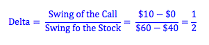
*A one dollar swing in the price of the stock causes a 1/2 dollar swing in the price of the call.
How much to borrow?
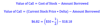
If we buy a call option with an exercise price of $50, we will end up with $10 next year if the stock price rises to $60. Therefore, in pricing our strategy, we need to hypothetically borrow an amount that will make the payoff of the borrow-and-buy strategy equal to the payoff of buying the call. If we buy one half of a stock, and the stock price rises to $60 next year, the value of our one half of a stock will be $30. This is $20 more than the value of the call. Therefore, we should borrow an amount today with a future value next year of $20. The present value of $20 (assuming a 10% discount rate) is $18.18 ($20/1.10).
Value of the call.
We know that if two strategies have an equal payoff at expiry their initiatial costs must be the same. Therefore, if we calculate the cost of buying the stock and the amount borrowed, we can find the price of the call.
The Black-Scholes Model
The delta hedging strategy shows us how to value an option with a two-state (binomial strategy) over a one-year time period. However, in the real world, there are more than two possibilities for the price of the stock one year from now. As a result, Black and Scholes set to work to derive a formula that could be used to value an option in the real world. The Black-Scholes formula relies on the fact that, while there might be numerous possibilities for the price of the stock over a year, the two-state assumption can be used when the time period is shorter. By calculated the price of a dynamic duplicating strategy, that is, a borrowing-to-buy strategy that changes from one instant to the next, the Black-Scholes model is able to calculate the price of a call in the real world using the same intuition that we use for our two-state delta strategy.
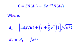
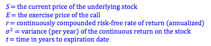
The value of a call option is a function of five variables, which are incorporated into the formula above.
In addition to these five parameters, the formula also incorporates the notation N(d), which stands for cumulative distribution function of the standard normal distribution. This represents the probability that a standardized, normally distributed, random variable will be less than or equal to d. We call this probability the “cumulative probability” and can find N(d) by calculating statistically the cumulative probability or by looking at a cumulative normal probability table.
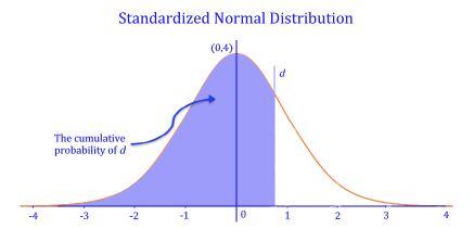
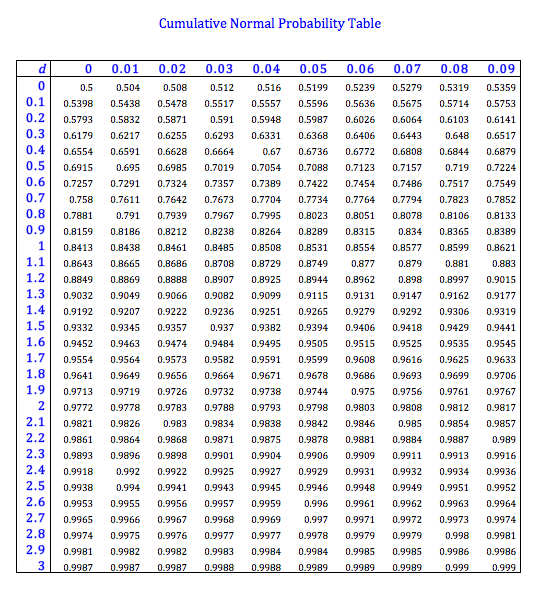
Photo by Maxwell Young on Unsplash
© BrainMass Inc. brainmass.com July 3, 2026, 10:53 am ad1c9bdddf