Spring-Mass-Dashpot System Simulation
Not what you're looking for?
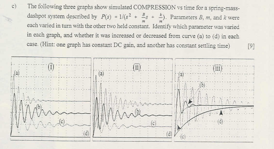
The attached graphs show simulated compression vs time for a spring-mass-dashpot system described by P(s) = 1/[s^2 + (B/m)s + k/m]. Parameters B, m, and k were each varied in turn with the other two held constant. Identify which parameter was varied in each graph, and whether it was increased or decreased from curve (a) to (d) in each case. (Hint: one graph has constant DC gain, and another has constant settling time).
Purchase this Solution
Solution Summary
The solution includes the calculations and MATLAB code. A spring-mass-dashpot system simulations are given. The expert analyzes the constant DC gains.
Solution Preview
% m is varied and B and k are fixed.
hold on;
%constant
B = 1;
k = 3;
%Vary
m = [20:20:80];
for i=1:4,
num = [1];
den = [1 B/m(i) k/m(i)];
sys = tf(num,den);
...
Purchase this Solution
Free BrainMass Quizzes
Architectural History
This quiz is intended to test the basics of History of Architecture- foundation for all architectural courses.
Air Pollution Control - Environmental Science
Working principle of ESP