Regress Dividend Payments

Solution Preview

I've attached two word documents with the SAS code and comments included. In the first excercise you are looking at the effects of male vs. female models, but more importantly you are looking at the effects from using AHE82 vs. AHE (which has been adjusted for inflation I suspect). The model with AHE fits much better. Also, look at the signs and magnitudes of the coefficients and consider their effect on the dependent variable.

In exercise two, you are looking at a plain vanilla OLS model and comparing it to a model with seasonal effects via dummy variables. This is a nice exercise to help understand the properties of time series data (i.e. seasonality and time trend issues).

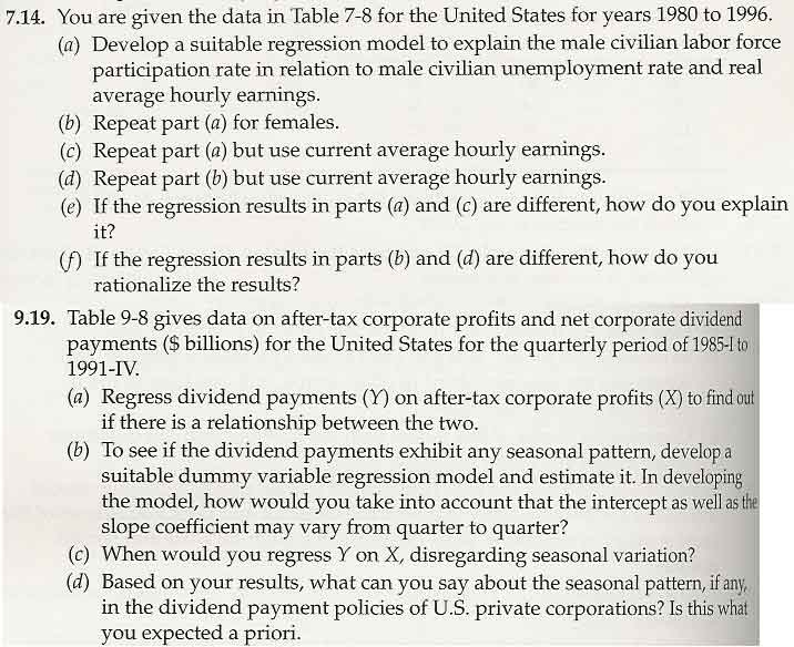
Exercise 7.14

SAS setup
DATA labor_1;
set labor;
run;

part A)
Here I am just looking at some descriptive stats for the data.

proc means data=labor_1 n mean median std var min max;
var clfprm clfprf unrm unrf ahe82 ahe;
run;

The MEANS Procedure

Variable N Mean Median Std Dev Variance Minimum Maximum
ƒƒƒƒƒƒƒƒƒƒƒƒƒƒƒƒƒƒƒƒƒƒƒƒƒƒƒƒƒƒƒƒƒƒƒƒƒƒƒƒƒƒƒƒƒƒƒƒƒƒƒƒƒƒƒƒƒƒƒƒƒƒƒƒƒƒƒƒƒƒƒƒƒƒƒƒƒƒƒƒƒƒƒƒƒƒƒƒƒ
CLFPRM 17 76.0941176 76.300 0.6859943 0.4705882 74.900 77.400
CLFPRF 17 55.8882353 56.600 2.5670709 6.5898529 51.500 59.300
UNRM 17 6.9117647 6.900 1.3896413 1.9311029 5.200 9.900
UNRF 17 6.8058824 6.600 1.2477332 1.5568382 5.400 9.400
AHE82 17 7.6105882 7.680 0.1655850 0.0274184 7.390 7.810
AHE 17 9.3700000 9.280 1.5229412 2.3193500 6.660 11.820
ƒƒƒƒƒƒƒƒƒƒƒƒƒƒƒƒƒƒƒƒƒƒƒƒƒƒƒƒƒƒƒƒƒƒƒƒƒƒƒƒƒƒƒƒƒƒƒƒƒƒƒƒƒƒƒƒƒƒƒƒƒƒƒƒƒƒƒƒƒƒƒƒƒƒƒƒƒƒƒƒƒƒƒƒƒƒƒƒ

Here's a quick look at the histogram of the dependent variable to check that it's normally distributed.
proc univariate data=labor_1;
histogram clfprm /anno=labor_1 normal(color=blue)
cfill=grey midpoints=73 to 79 by .1;
run;

Here are is another graphical test for normality of the dependent variable.
proc univariate data=labor_1 noprint;
var clfprm;
qqplot / normal(mu=est sigma=est color=red);
run;

Again we check for a quadratic relationship between the dependent variable and the independent ...